Joules, watts, tonnes of CO2, kilowatt-hour, you name it. If you have read any articles about energy consumption, you have probably come across these units. This medley of units can sometimes make it difficult to grasp key concepts in your reading. These units are not necessarily representing the same concept. For example, power (measured in watts) is different from energy consumption (measured in joules). Before diving into green software, we ought to be comfortable with the jargon. This article serves as a go-to source of truth for energy-related metrics.
There is no doubt that energy efficiency is a concern that is growing by the day among software engineers. Traditionally, energy efficiency has been a requirement for software running on devices with limited energy capacity – for example, mobile applications – or to cut down the electricity bill in massive data centres across the globe. Thankfully, concerns about environmental sustainability are becoming a top priority in our society, and the tech sector is not an exception.
Also, driven by personal interests, tech workers are becoming more interested in being part of organisations that do care about the environmental sustainability of their operations. Yet, literature around software energy efficiency can be difficult to grasp. Personally, we find it difficult to compare all the different energy metrics across different articles. No wonder, to make things easier, many reports have been using measures that resemble day-to-day concepts. For example, one bitcoin transaction is equivalent to more than one million VISA transactions (as of 2021). This is easier to grasp than saying that one Bitcoin transaction requires more than six giga-joules (6,000,000,000J). Well, six giga-joules sound massive anyway, but you get the point 🏭.
In this article, we will go on a tour around energy consumption metrics to help you understand the jargon and make sense of all the numbers. While it is not an exhaustive list, the most occurring categories concerning energy consumption, i.e. energy, power, batteries and carbon, are highlighted below. Hopefully, after reading this, you can tackle any article using energy consumption metrics without much effort! 🥷
Energy
Energy is often referred to as work: for example, in electricity, energy is the work required to move charged particles. The International System of Units (SI) defines joule (J) as the standard unit of energy. It is also the most common unit of energy used in scientific literature.
Another common unit is kilowatt-hour (kWh). For example, it is used to report household electricity consumption. Kilowatt-hour represents the exact same parameter as joule but in a much higher order of magnitude. Kilowatt-hours can be easily converted to/from joules as follows:
\[1\text{kWh} = 3,600,000\text{J}\]For example, saying that 1 bitcoin transaction requires more than 6 giga-joules ($6 \cdot 10^9 \textnormal{J}$) is similar to saying that it requires more than 1667kWh (approximately).
Power
When measuring energy consumption, it is also common to talk about power consumption. Briefly, power represents the amount of work being done by a unit of time. For example, using standard SI units, 1 unit of power is equivalent to 1 joule per second. Instead of joules per second, we call it watts (W) in memory of the Scottish inventor James Watt.
Not surprisingly, some energy profiler tools report power consumption instead of energy consumption.
For example, the tools Powerstat and PowerTOP, mentioned in a previous post regarding some state-of-the-art tools to measure energy consumption from your computer, report the (average) power consumption.
Using power units instead of energy units is useful in particular scenarios. Imagine that we want to measure the energy consumption of reading a book on a device. Saying that reading a book spends 10J does not say much about its energy efficiency – the user could be reading for 1 minute or 10 minutes. In those cases, it makes sense to talk about power consumption. On the other hand, if we talk about a Bitcoin transaction, we really don’t want to talk about power – we should rather be talking about the total energy consumption.
Power consumption is often not what matters
In a software project, energy consumption is usually the go-to parameter. We want to analyse the project by use case: for example, the energy consumption of applying a filter to a photo, uploading a file to the server, etc. Hence, as a rule of thumb, energy consumption is the parameter we should be reporting when testing energy in software projects. To compute energy consumption using power consumption, we need to factor in the duration of the execution. Given the average power consumption ($P_{avg}$), and the duration of the execution ($\Delta{t}$), the energy consumption ($W$) is computed as follows:
\[W = P_{avg} \dot{} \Delta{t}\]Nevertheless, the above function only works when the power consumption is constant. It works fine when we deal with the average power consumption, but it does not work when we have a stream of power consumption measurements. Power monitors, depending on their precision, might collect several power samples per second. Hence, before computing the total energy consumption, one needs to combine and process power data and respective timestamps.
The process is straightforward but it is important that we understand the underlying concepts. Energy consumption ($W$) is the integral of power consumption ($P$) over the interval of time needed ($[t_0, t_n$]) to execute a given software operation:
\[W=\int_{t_0}^{t_n}P(t) dt\]As always, it is easier to grasp ideas from visualisations. The figure below depicts a line plot with power on the y-axis and time on the x-axis. The integral – i.e., energy consumption – is basically the grey area under the line and between the beginning ($t_0$) and the end ($t_n$) of the execution.

Figure 1: Plot of power consumption over time. The area in gray is equivalent to the energy consumption between $t=1\text{s}$ and $t=9\text{s}$. View source.
Yet, no power monitor will give us the precise mathematical function to compute the exact energy consumption. In the best-case scenario, it retrieves a sequence of the values of power consumption with respective timestamps. Hence, instead of a line, we actually have a sequence of points, similar to the dots in the plot below:

Figure 2: Scatter plot of the power samples that were collected by a power monitor. The black dots represent the power measurements, which were collected at the rate of 1 sample per second. The dashed line represents the real power consumption. View source.
It is up to us to connect the dots and compute the energy consumption – i.e., the area under the curve:

Figure 3: Plot showing how the energy consumption, in the grey area, can be extracted from a sequence of power measurements. View source.
In this figure, the area under the curve is not exactly equal to the one in the first figure. There will always be an error stemming from this approximation which can be reduced by increasing the sampling rate – i.e., the number of power measurements we collect per second, measured in hertz ($\text{Hz}$). In the example of the figure, the sample rate is $1\text{Hz}$. Power monitors such as the Monsoon Power Monitor can operate in $5000\text{Hz}$. Yet, approximation errors will always be part of measuring energy consumption, and that is fine.
If we take a closer look at the plot, we observe that the area under the curve is approximately equivalent to the sum of multiple trapezoids. Hence, to estimate the energy consumption we simply have to sum the areas of the trapezoids. First, let’s remember the area (A) of a trapezoid:

In our case, $a$ and $b$ would be two subsequent power measurements – $P_{t_n}$, $P_{t_{n+1}}$ – and $h$ would be the elapsed time between the two measurements – $\Delta{}t = t_{n+1} - t_{n}$:
\[A= \frac{P_{t_n}+P_{t_{n+1}}}{2}\cdot{}\Delta t\]If we go back to the data from Figure 3, the area of the first trapezoid, within the time interval $t=1\text{s}$ and $t=2\text{s}$ is calculated as follows:
\[A= \frac{3.5\text{W}+2.0\text{W}}{2}\cdot{}1\text{s} = 2.75\text{J}\]To calculate the total energy consumption between $t=1\text{s}$ and $t=9\text{s}$, we simply have to sum all the areas of the 8 trapezoids in Figure 3.
This is basically the mathematical approach to approximate an integral – the Trapezoid rule. It is formulated as follows:
\[\int_{t_0}^{t_n}P(t) dt \approx \frac{\Delta t}{2} [ P(t_0) + 2P(t_1) + 2P(t_2) + ... + 2P(t_{n-1}) + P(t_n) ]\]The formula looks odd but scientific software libraries make it super simple to calculate. Here is an example in Python, using the numpy package:
"""
    Args:
        power_sample (List[float]): List of power consumption values.
        timestamps (List[float]): List of corresponding timestamps for the power consumption values.

    Returns:
        energy_consumption (float): Total energy consumption calculated using the trapezoidal rule.
"""

import numpy as np
energy_consumption = np.trapz(power_sample, timestamps)
Energy Delay Product (EDP)
The Energy Delay Product (EDP) is another metric used for measuring energy consumption but with the aim to balance both energy efficiency and speed. It is defined as the product of energy consumption ($E$) and execution time ($t$) including an exponential weight $w$ to penalize for slow execution time more adequately. The exact formula is as follows (note: $\Delta P$ is the energy consumption per unit of time):
\[EDP = E \cdot t^{w} = (\Delta P \cdot t) \cdot t^{w}\]This metric penalizes simply running software on a low-power mode of the CPU, making execution slow but substantially more energy-efficient, by giving more importance to runtime. Ultimately, the goal is low-energy and fast runtime applications, thus, using this metric for comparisons is recommendable. Most common is $w = 1$, resulting in quadratic time, but it can also be any other positive value depending on the scenario: a higher value (e.g. 3) works great for performance efficiency. This can be especially useful for assessing the energy efficiency of programming languages. While Java is known for its high performance, its relatively slow compile time is penalized heavily using EDP and resulted in Java being one of the weakest-performing programming languages according to the work of Georgiou et al. (recommendable read if you are interested in the complete overview of the EDP comparisons between the most used programming languages).
Milliampere hour (mAh)
If you have ever worried about the battery life of your mobile devices, you have probably come across this unit: milliampere hour, abbreviated as $\text{mAh}$. This is not a unit of energy. It is rather a unit to measure capacity, a different parameter. To convert capacity to energy consumption we have to multiply the capacity by the voltage. For example, if you have used $1000\text{mAh}$ from your battery to run a smartphone device operating at the voltage of $3.8$ volts, the total energy consumption would be as follows:
\[W = 1000\text{mAh} \times 3.8\text{V} = 3800\text{mWh} = 3.8\text{Wh} = 3.8 \times 3600 \text{J} = 13680 \text{J}\](Note that the calculation above would have been much simpler if $\text{mAh}$ was an SI unit.)
It would be much simpler if batteries could also report the amount of work (i.e., energy) one can do with a single battery cycle in joules. The problem is that, contrary to the example above with $3.8\text{V}$, the voltage is continuously decreasing throughout a battery cycle. I.e., when the battery is fully charged its voltage is higher than when it is, for example, at 60% of full capacity. The continuous change of voltage throughout a charge cycle makes the comparison of batteries based on energy units, extremely difficult and imprecise. In conclusion, we have to live with $\text{mAh}$.
Another fun fact, as mentioned above, $\text{mAh}$ is not the SI unit for capacity. The SI unit for capacity is coulomb, abbreviated as $\text{C}$. A single $\text{mAh}$ is equivalent to $3.6\text{C}$, which is roughly within the same order of magnitude. Using SI units makes it much simpler when we need to perform calculations. However, $\text{mAh}$ is found to be most convenient, as it is much more typical for batteries or circuit measurements to report values in $\text{mA}$ and expected battery lifetime is easiest to grasp in hours for consumers. Therefore, the common order of magnitude behind $\text{mAh}$ has made it more popular than its SI unit equivalent.
Percentage
The battery percentage, i.e. the present battery capacity as a percentage of maximum capacity, is the most common way to communicate the remaining battery life users have left. In scientific papers, this is usually denoted as State of Charge (SoC). Most devices use the voltage of the battery to compute their battery level percentage. Overall, the battery percentage is not a straightforward concept due to the continuous change in voltage throughout a battery’s (dis)charge cycle causing mysterious behaviour at times.
Contrary to popular belief, the relationship between voltage and battery percentage is not linear. While a lot of effort is dedicated to making the battery voltage remain constant until it is close to fully discharged, the voltage curve can vary between different battery chemistries, temperatures, and discharge rates. This explains why sometimes your phone’s battery percentage might seem to drop quickly at the beginning and then slow down, or it might suddenly drop from 20% to 0%. These changes in voltage can also be affected by the type of charger used, the age of the battery, and the type of device. As a sample to visualise all of this, Figure 4 shows the discharge characteristics of a Li-ion battery by Panasonic with excellent load capabilities.
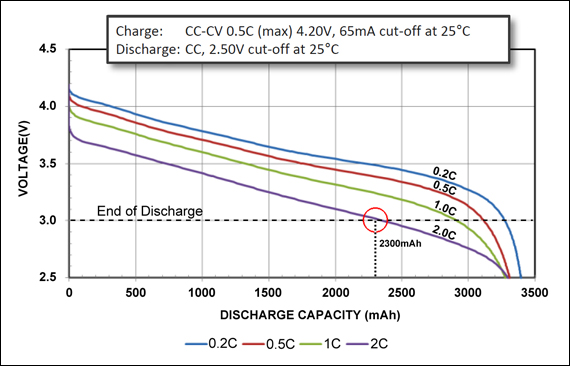
Figure 4: Discharge characteristics of a Li-ion Energy Cell by Panasonic. This particular energy cell is made for portable computing and illustrates a particularly linear change in voltage. View source.
To make things more complicated, some devices use a combination of voltage, current, and temperature measurements to estimate the battery level more accurately. This is because the voltage of a battery can change even when it’s not being used, for example, due to self-discharge or temperature changes. So, the next time your battery seems to be draining quickly, don’t blame the device – even the most advanced batteries are subject to the laws of science!
Depth of Discharge (DoD)
Simply put, battery lifespan is the amount of time your battery lasts until it needs to be replaced – something you want to delay for as long as possible 💸. Lithium-ion batteries, which are used in most smartphones and laptops, have a limited number of charge cycles before they start to degrade. A charge cycle is defined as the process of fully charging a battery and then discharging it to a specific percentage. Lithium-ion batteries typically last for 300-500 charge cycles before their capacity starts to decline.
The Depth of discharge (DoD) is a critical factor that affects battery lifespan. It refers to the percentage of a battery’s maximum capacity that has been discharged. A deep discharge is a DoD of at least 80%. Deep discharges can significantly reduce the number of charge cycles a battery can undergo. Therefore, it’s important to avoid deep discharges whenever possible. Instead, try to keep the depth of discharge between 20% and 80%. This means charging your device when the battery level drops to 20% and unplugging it when it reaches 80%.
Additionally, leaving your device plugged in for extended periods can lead to overcharging, which can damage the battery and reduce its lifespan. To combat these issues, some companies such as Apple already developed smart features to combat battery harm. For example, leveraging machine learning to recognize your (overnight) charging habits and follow an adjusted charging schedule that finishes shortly before the predicted first usage. If you can, it is also recommended to remove certain device cases and covers while charging, as they might cause excess heat leading to battery degradation.
Carbon
Greenhouse gas emissions due to human activities are at the heart of the recent heating of Earth’s climate system – the so-called phenomenon of Global Warming.
The greenhouse gases that most affect global warming are Carbon Dioxide (CO2) and Methane (CH4). Yet, many other gases are also part of the issue – a total of 7 – as mentioned by the Kyoto Protocol: Nitrous Oxide (N2O), Hydrofluorocarbons (HFCs), Perfluorocarbons (PFCs), Sulphur Hexafluoride (SF6), and Nitrogen Trifluoride (NF3).
By reducing the energy consumption of software we are reducing the emission of greenhouse gases stemming from the production of electricity used to power the system. However, the environmental impact of 1 Joule is not the same in every system. Depending on the power source, the environmental impact of software will vary. For example, systems powered by solar panels will have much fewer gas emissions than systems powered by fossil-fuel plants. Thus, it is important to remember that energy efficiency and carbon efficiency are not equivalent.
Hence, instead of talking about energy consumption, many articles report its impact in terms of gas emissions. This is particularly useful when we move from a software-level perspective to the level of the infrastructure. At the software level, improving energy efficiency is the de facto approach to reducing gas emissions. On the contrary, at the infrastructure level, there are many more issues besides energy consumption (electricity provider, e-waste, cooling equipment, etc.).
Hence, we resort to the carbon footprint to measure and communicate greenhouse gas emissions. It is formally named as carbon dioxide equivalent, commonly abbreviated as CO2-eq, CO2eq, CO2-e, and CO2e. It is measured in mass units, with different orders of magnitude depending on the context:
- billion metric tones of carbon dioxide equivalent ($GtCO_2eq$) in country-wide or planet-wide studies
- million metric tonnes of carbon dioxide equivalent ($MMTCDE$ or $MMT CO_2eq$)
- kilograms of carbon dioxide equivalent ($\text{kg}CO_2eq$). By default, use this one, as it is the SI unit for mass.
And because when we talk about gas emissions we are not only talking about carbon dioxide, we have to sum the emissions of all greenhouse gases. However, not all gases have the same impact on the environment. For example, $1\text{kg}$ of CH4 is estimated to be 21 times more harmful to the environment than $1\text{kg}$ of CO2.
Hence, we used a weight function that combines all gas emissions into their carbon dioxide equivalent. It relies on the estimation of the impact of greenhouse gases on global warming over a period of 100 years when compared to carbon dioxide. This is a metric called 100-year global warming potential and abbreviated as 100-GWP. The table below shows the 100-GWP of the most common greenhouse gases.
| Greenhouse Gas | 100-GWP |
|---|---|
| Carbon dioxide $CO_2$ | $1$ |
| Methane $CH_4$ | $21$ |
| Nitrous oxide $N_2O$ | $310$ |
| Sulphur hexafluoride $SF_6$ | $23900$ |
In sum, the weight function to calculate the $CO_2eq$ looks as follows:
\[CO_2eq = \sum_{g\in GHG}({GWP_{g}\cdot{} m_{g}}),\]where $GHG$ is the set of all greenhouse gases, $GWP_g$ is the 100-GWP of a given gas $g$, and $m_g$ is the total mass of gas $g$ that was emitted.
As an example, imagine that to run our software system our electricity provider emits $1000\text{kg}$ of $CO_2$, $20\text{kg}$ of $CH_4$, $5\text{kg}$ of $N_2O$, and $0\text{kg}$ of the remaining greenhouse gases. Our $CO_2eq$ would be computed as follows:
\[CO_2eq = GWP_{CO_2}\cdot{} m_{CO_2} + GWP_{CH_4}\cdot{} m_{CH_4} + GWP_{N_2O}\cdot{} m_{N_2O}\\ = 1 \times 1000 + 21 \times 20 + 310 \times 5 \\ = 2670\text{kg}\]Please, note that the 100-GWP is an estimation. One can only speculate about the impact of some gas on global warming. Hence, some of these values are sometimes presented as a range or may vary slightly amongst different sources. Our go-to source is The Intergovernmental Panel on Climate Change from the United Nations. Find the reference at the bottom of the article (Forster et al., 2007). It includes an extensive list of GWPs, including HFC and PFC gases, which are missing in the table presented above.
Carbon Intensity
The carbon intensity is the amount of carbon dioxide equivalent that is emitted per unit of energy consumed. It is commonly measured in $CO_2eq/kWh$ or $CO_2eq/MWh$. It is a useful metric to properly compare the carbon footprint of various energy systems and sources, as the energy consumption of a given system will vary depending on the power source. For example, a slow system that is powered by a solar panel can have the same footprint as a fast system that is powered by a coal plant – carbon intensity allows us to make a distinction between the two. Of course, the goal is to have both a low carbon intensity and a low energy consumption.
Note, carbon intensity can vary heavily due to several external factors. For example, the amount of $CO_2eq/kWh$ emitted differs substantially by the time of day and location due to the types of generation (wind, solar). When demand is higher than the existing power in the electricity grid, renewable-based power plants cannot adapt to demand and we need a power plant that is able to scale up to that demand. This is usually done by fossil-based power plants, also called marginal power plants. The problem is that marginal power plants do not scale down to zero. There is always a minimum carbon that needs to be emitted, even if there is a lot of renewable energy in the grid. Therefore, it is of key importance to account for the marginal carbon intensity: the increase or decrease in carbon emissions in the electrical grid, in response to an infinitesimal increase/decrease in power demand/supply.
One way to account for volatile marginal carbon intensity is by making your system carbon-intelligent with regard to the datacentres used for your energy consumption. Google sets a great example by having a sophisticated pipeline in place for managing this, but it is actually rather achievable for any small company or developer using the API called ElectricityMaps. This API provides carbon data from different countries and allows anyone to consume electricity at more sustainable times, to estimate savings leveraged with carbon-aware consumption, and to report on their carbon footprint reduction.
Carbon Efficiency
While carbon intensity is one way to measure the effectiveness of carbon usage, there are more ways to go about this. Scaling an amount of carbon dioxide equivalent to another factor is generally referred to as carbon efficiency and has multiple forms. Below, the two most popular are listed. Though arguably controversial, money (revenue) can be seen as a byproduct of created value. In corporate settings, this is the most common measurement used to reflect on carbon usage and is typically referred to as carbon efficiency. It can be calculated by dividing the total sum of $CO_2eq$ by the sum of all revenues. In the lifecycle assessment of products, it is common to look at the amount of carbon dioxide equivalent that is emitted to produce a given product (embodied carbon). Putting operational carbon in perspective with embodied carbon allows for a clearer outlook on the relative impact of software based on the utilised hardware.
Wrap-up
The tour has finished! 🚌 After visiting the most common energy consumption jargon and metrics, you are hopefully more familiar with these concepts by now. Furthermore, you can start utilizing this knowledge by designing or using best practices and helpful tools. This is of key importance for environmental sustainability: as our reliance on technology continues to grow, so does the demand for energy to power it. In a different article, more awareness will be created for this by diving into certain software engineering guidelines you could adopt to reduce or optimize carbon emissions.
If you have any questions or miss information about some specific metric, please drop an email or send a message on Twitter.
Useful resources 📚
If you want to learn more about the topics described above, here are some follow-up pointers you should not miss:
- The Principles of Sustainable Software Engineering. A nice course designed by Asim Hussein at Microsoft covering concepts such as carbon, carbon intensity, embodied carbon, and so on.
- Forster et al. (2007). Changes in Atmospheric Constituents and in Radiative Forcing. Climate Change 2007: The Physical Science Basis. Cambridge University Press.
- Why are milliampere hours commonly used instead of watt hours to measure battery capacity?. Interesting discussion about the usage of $\text{mAh}$ instead of joules to report battery specs.
- A Guide to Understanding Battery Specifications. Guide with in-depth coverage of more specific battery jargon.
@misc{cruzbekker2023energyunits,
  title = {All you need to know about Energy Metrics in Software Engineering},
  author = {Luís Cruz, Philippe de Bekker},
  year = {2023},
  howpublished={\url{http://luiscruz.github.io/2023/05/13/energy-units.html}},
  note = {Blog post.}
} © 2023 – onwards by Luís Cruz. Licensed under the