Back to all projects

Measuring the Energy Impact of Mixed Precision on Convolutional Neural Network Training

Emre Çebi, Aadesh Ramai, Noah Tjoen, Andrea Vezzuto.

Group 30.

We measured the energy impact of mixed precision on the training process of a convolutional neural network. Our findings demonstrate that, compared to the default 32-bit floating point accuracy, mixed precision reduces energy consumption by more than 12%, while only sacrificing 1% accuracy in test accuracy.

Introduction

Neural networks have become the backbone of a large push for artificial intelligence in recent years. These models typically contain millions of optimisable parameters, which, although highly flexible, are computationally expensive to train. While performance metrics such as classification accuracy dominate evaluation, the substantial energy consumption of training these systems is often overlooked. As such, modern machine learning models can carry a high environmental cost.

To improve the computational efficiency of deep learning models, mixed precision training can reduce memory usage while maintaining similar classification performance. When mixed precision training is enabled, most computations, such as matrix multiplications and convolutions, are computed in 16-bit floating point precision instead of the standard 32-bit. This reduction in numerical precision decreases the memory required to store model parameters, gradients, and intermediate activations, allowing more data to be processed within the same hardware constraints. These factors suggest that mixed precision training may also decrease the overall energy consumption associated with training neural networks. However, while reductions in memory usage are well established, the extent to which these translate into measurable energy savings remains an open question.

To investigate this, we measure the energy impact of mixed precision on the training process of a convolutional neural network (CNN) with EnergiBridge. The CNN, implemented in TensorFlow, is adapted from one that is publicly available on Kaggle¹. The dataset on which it is trained is the CIFAR-10 dataset², which consists of 60.000 color images of \(32 \times 32\) pixels with 3 channels (RGB), evenly distributed across 10 classes.

After 60 training runs of our CNN on the CIFAR-10 dataset, our results indicate that enabling mixed precision significantly reduces power consumption, yielding an average energy saving of approximately 12% while maintaining comparable test accuracy. All code relating to the CNN training and results analysis can be found on GitHub³.

Methodology

The CNN used in this experiment is a simple convolutional architecture, consisting of:

• Two convolutional blocks with 128 filters followed by pooling and dropout,
• Two convolutional blocks with 128 filters followed by pooling and dropout,
• Two convolutional blocks with 256 filters followed by pooling and dropout,
• A fully connected layer with 1024 units,
• A final softmax classification layer with 10 output units.

When mixed precision is enabled, the global policy is set to mixed_float16 using TensorFlow’s mixed precision API. However, the final dense classification layer is explicitly forced to use float32 precision. This is done to preserve numerical stability in the final softmax activation and loss computation. The model is trained on 50,000 images of the aforementioned CIFAR-10 dataset, while the remaining 10,000 images are reserved for testing and evaluation.

To ensure reproducibility and fairness in the comparison between the training methods, the experiment is fully automated using a Python (version 3.11) orchestration script. The script fixes the random seed to reduce stochastic variation, executes 10 runs for each configuration, and randomises their order to avoid systematic bias caused by thermal drift or background system load. Furthermore, a 5-minute CPU warm-up phase is performed prior to the measurements to stabilise hardware conditions, and a 2-minute cooling period is inserted between runs to minimise interference across consecutive executions. Additionally, several measures have been taken to ensure minimal impact of external factors during the experiment. Physically, the machine was kept in a temperature-controlled environment and positioned away from external heat sources. On the software side, auto-brightness was disabled, the internet connection was turned off, notifications were disabled, and only the terminal required to execute the script was left running.

To measure energy consumption during training, we integrated EnergiBridge into the experimental pipeline. EnergiBridge is executed as a separate background process at the start of each run and records system-level energy metrics while the training procedure is carried out. The orchestration script programmatically starts EnergiBridge immediately before model training and terminates it once training completes, ensuring that only the relevant execution window is measured. The energy measurements are then exported to CSV files and stored alongside the accuracy metrics for each run.

Results

In this section, we outline some of the key results obtained from our experimental runs. These were performed on an M2 Ultra machine running MacOS 26.3, with 16 performance cores, 8 efficiency cores and 128GB of unified memory. The PC was connected to a 27-inch Apple Studio Display (5120 by 2880 resolution) and wirelessly to an Apple wireless keyboard and mouse via Bluetooth. Overall, we compare single-precision floating-point (FP32) training to mixed precision training across several facets: energy consumption, stability, and testing accuracy. It is worth noting that FP32 training is the default precision when training neural networks, and thus serves as a baseline on which to compare mixed precision training. Furthermore, one of the 30 FP32 runs were excluded after being identified as an outlier based on a predefined z-score threshold of 3 (that is, more than three standard deviations from the mean total energy consumption). Given the otherwise low variance across runs, this observation was considered non-representative and was removed to avoid an inaccurate influence on aggregate statistics.

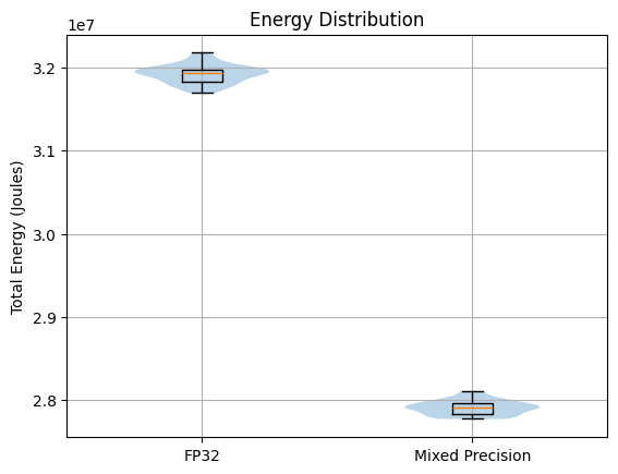
Figure 1: Violin plots overlaid with box plots, showing the total energy consumption accumulated over the different runs of mixed precision and FP32 model training.

Figure 1 presents violin plots overlaid with box plots illustrating the distribution of total energy consumption for both FP32 (standard precision) and mixed-precision configurations. The violin plots seem to roughly suggest a normal distribution for both training types. A Shapiro–Wilk test confirms that there is no significant deviation from normality for either group: (\(p_{\text{FP32}} = 0.59\), \(p_{\text{mixed}} = 0.27\)). As such, our analysis can rely on parametric methods that assume an underlying normal distribution of the data. From the box-plots, it is immediately clear that mixed precision training consistently consumes less energy across the different runs compared to FP32. In fact, mixed precision consumed approximately \(2.80 \times 10^{7}\) Joules per run, while FP32 training consumed approximately \(3.18 \times 10^{7}\) Joules per run. This corresponds to a mean energy reduction of roughly 12–13% when using mixed precision. Furthermore, the energy consumption of runs seems fairly consistent across both training modalities due to the relatively small whiskers on the box plots. This is confirmed by small coefficients of variation: \(0.36\%\) and \(0.32\%\) for FP32 and mixed precision, respectively. We can further quantify the difference in total energy consumption between FP32 and mixed precision via an independent two-sample \(t\)-test, which reveals a highly significant difference in total energy consumption (\(t = 151.43\), \(p < 10^{-75}\)). Additionally, the computed effect size is extremely large (Cohen’s \(d = 39.44\)), indicating that the distributions are almost completely separated and that the observed reduction in energy is not only statistically significant but also rather substantial.

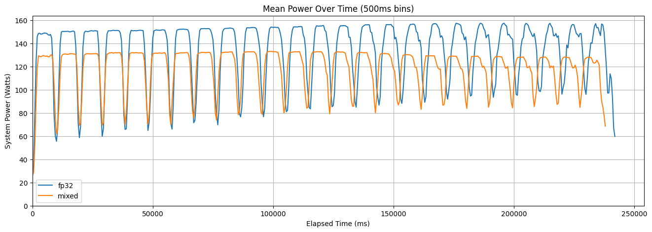
Figure 2: Mean power usage across all runs of mixed precision and FP32 training over time.

Having established that mixed precision consumes less energy compared to FP32 training, we aim to deepen our understanding of how exactly this is obtained. Is system power during training consistently lower for mixed precision? Or does mixed precision simply take less time to train? To this end, Figure 2 shows the mean system power usage across all runs of the two training modalities over time. Given that our power usage samples do not always perfectly align (the delta between individual measurements varies between \(199\)ms and \(209\)ms), we have chosen to aggregate the data points into \(500\)ms bins and calculate the mean within them. Generally, both FP32 and mixed precision seem to take approximately the same time to train. In fact, the mean training times are \(2.39 \times 10^{5}\) and \(2.36 \times 10^{5}\) for FP32 and mixed precision training, respectively. This indicates that the energy savings are not primarily derived from shorter training duration. Instead, the difference is driven by consistently lower system power usage throughout training when using mixed precision. Beyond the overall level difference, the temporal trends also demonstrate some interesting differences. Mixed precision exhibits a slight but steady decrease in mean system power as training progresses. In contrast, FP32 shows a gradual increase in power consumption over time. This divergence suggests that the two modalities interact differently with system resources as training progresses.

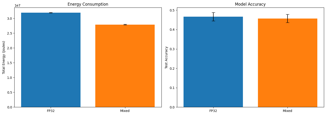
Figure 3: Energy consumption and accuracy comparison between FP32 and mixed precision training.

Metric	FP32	Mixed Precision
Energy Usage (J)	3.19 × 10⁷ ± 1.13 × 10⁵	2.79 × 10⁷ ± 8.91 × 10⁴
Model Accuracy	0.467 ± 0.022	0.457 ± 0.021

Table 1: Comparison of the energy usage and model accuracy of FP32 and Mixed Precision training. Values are reported as mean \(\pm\) standard deviation.

While the power–time analysis clarifies what the energy savings can be attributed to, it does not yet address whether this reduction comes at the cost of model performance. To evaluate this trade-off, Figure 3 presents a side-by-side comparison of total energy consumption and test accuracy for FP32 and mixed precision training, and visually summarises the numerical results reported in Table 1. Clearly, the drop in energy consumption is quite substantial and consistent across runs, while the model accuracy decreases slightly. Overall, paired with such a large decrease in energy usage, a small drop in performance becomes negligible. Test accuracy decreases slightly from \(0.467\) to \(0.457\), representing an absolute difference of \(0.01\) (that is, one percentage point). Given the overlapping standard deviations (\(\pm 0.022\) and \(\pm 0.021\)), this reduction appears small relative to the variability observed across runs. In fact, the difference between test accuracy is not statistically significant (\(t = 1.71\), \(p = 0.093\)). The effect size (Cohen’s \(d = 0.45\)) is moderate, suggesting a small-to-medium practical difference, but given the lack of statistical significance, we can consider the accuracies effectively comparable. Combining this with predictive performance, mixed precision is more energy-efficient, consuming on average \(6.11 \times 10^{7}\)J per accuracy point compared to \(6.85 \times 10^{7}\)J per accuracy point for FP32. This further supports the case that mixed precision saves energy without meaningful accuracy loss.

Discussion

The results of our experiment provide a fairly consistent picture: mixed precision training reduces total energy consumption without significantly affecting the test accuracy of the model. In this section, we interpret these results in greater detail and aim to explain the impact of mixed precision on neural network training.

We first consider the nature of the observed energy savings. The 12-13% reduction in energy consumption aligns well with our initial expectation that mixed precision would primarily lower instantaneous power consumption rather than dramatically shorten training time. In fact, as shown in Figure 2, the wall-clock training durations were nearly identical. This indicates that the energy savings are not attributable to faster convergence or fewer iterations, but stem from consistently lower mean system power usage throughout training. This behaviour is consistent with the advantages of lower-precision arithmetic. By reducing numerical bit-width, mixed precision decreases memory traffic and per-operation switching activity, thus lowering the energy required for each computation. Therefore, the total computational workload remains unchanged, but it is executed more energy-efficiently at the hardware level. Over a training cycle, this sustained reduction in average power directly translates into the observed decrease in total energy consumption with approximately equal wall-clock durations.

The stability of this energy reduction further strengthens our conclusions. The total energy consumption for both training modalities followed an approximately normal distribution (Figure 1), as confirmed by the Shapiro-Wilk tests. This behaviour is expected: while random initialisation affects optimisation trajectories and final accuracy, it does not substantially change the computational workload under fixed hyperparameters. The extremely small coefficients of variation (CV \(< 0.4\%\)) suggest that hardware-level fluctuations, such as thermal noise, introduce only minor Gaussian variation, and validate our experimental controls.

Analysing the behaviour of mixed precision throughout the training process more closely, we can observe that both the training models exhibit periodic power drops (see Figure 2). These fluctuations are consistent with the natural compute-communication cycle in the CNN training iterations. Each training step alternates between compute-intensive phases with high power requirements (forward/backward pass, convolutions, etc.) and comparatively lighter communication phases with a noticeable power drop (weight updates, batch normalisation), where the operations mainly wait on memory I/O. The synchronised timing of these drops across both precision modes further confirms that they are derived from the same training loop structure, rather than precision-specific behaviour.

Furthermore, the minor test accuracy reduction observed in our experiments reflects the expected FP16 numerical limitations. Compared to FP32, FP16 uses fewer bits to represent each number, thereby reducing the accuracy with which weights, gradients, and activations can be stored. In turn, this increases rounding errors and reduces the dynamic range of representable values, meaning that very small gradient updates may be truncated or large values may require scaling. While mixed precision techniques, such as loss scaling and selective use of FP32 accumulators, compensate for some of these effects, small numerical differences may accumulate over many iterations, leading to a small drop in the final model accuracy. In most real-world applications, a 1% decrease in accuracy is negligible compared to a 12% increase in energy savings. However, in safety-critical applications, such as medical diagnostics, this very drop may still be considered to be critical. Therefore, the suitability of mixed precision depends on the use case and its tolerance to small accuracy trade-offs.

Before concluding, it is worth briefly addressing the removal of one FP32 run identified as an outlier, which exceeded a z-score threshold of 3 in total energy consumption. Given the extremely tight clustering of all other runs, this deviation is most plausibly attributable to an external disturbance (e.g., background system activity or transient hardware behaviour) rather than a systematic effect.

Conclusion and Future Work

Overall, our experiments demonstrate that mixed precision training can substantially reduce the energy consumption of training a convolutional neural network on the CIFAR-10 dataset, achieving a 12–13% decrease compared to standard FP32 training. This reduction is mainly driven by consistently lower system power usage rather than shorter training times, highlighting the efficiency benefits of lower-precision arithmetic and reduced memory traffic on modern hardware. Crucially, this energy saving comes with only a small and statistically insignificant drop in test accuracy, indicating that mixed precision is a practical approach for improving computational efficiency without compromising model performance.

The main limitation of the study is the unmeasured baseline power drawn by external peripherals such as the display, keyboard, and mouse, which were not captured by EnergiBridge. This means that while our measurements accurately reflect the energy consumed by the computational modules, they do not represent the total energy footprint of the system, therefore slightly underestimating real-world energy use. Furthermore, due to the limited time allocated for the study, we only computed our results on a single machine and one machine learning architecture. Therefore, extending our analysis to larger and more complex models, as well as different hardware, could provide wider insights into the generalisability of mixed precision for energy-efficient machine learning. In the future, it may also be valuable to investigate even lower-precision formats, such as 8-bit floating point, to explore whether further energy reductions are achievable while maintaining similar levels of accuracy.

Back to all projects