The Effect of Different Power Profiles on Energy Consumption and Runtime Performance in Machine Learning Applications
Rover van der Noort, Martijn Smits, Remy Duijsens, Dajt Mullaj.
Training neural networks is a daily task for AI engineers. In this study, we evaluate the effects of different power profiles on the performance and energy consumption of a neural network training benchmark. Our results show that the power-save profile causes the benchmark to use significantly less energy than the other power profiles. The difference in runtime is statistically significant but in absolute measure not practically relevant for this use case.
Introduction
Climate change is an important research topic and specifically, in the field of computer science the problem of massive power consumption persists [1, 2]. Recently many new solutions have appeared, which try to tackle this problem in a variety of ways [1, 2, 6, 9]. Popular operating systems (OS) have introduced powersaver settings as built-in features, which enable any user to activate them. It is however not directly clear how much energy these profiles save or how it affects the performance of a system.
The popularity of Machine Learning (ML) models has increased parallel to the interest in sustainability [3, 7]. However, generally, these models require large quantities of energy to train and deploy [3, 5, 7, 8]. It is therefore important to create a sustainable mindset for current and new ML engineers because they can significantly reduce the power consumption of their whole pipeline by choosing the right implementation details [7, 9].
TensorFlow is a widely used open-source library to create and deploy ML models. Perfzero offers a benchmark framework to test a system’s performance for ML computations. Although this benchmark does not cover the whole pipeline of ML engineering, it can show the effect of a general ML task and give an indication of any impact on power consumption and performance.
This study investigates the impact of the Ubuntu Power Profiles on the benchmark framework for TensorFlow and could show ML developers the impact of powersaver methods. This study elaborates on the studied libraries and how they will be tested, followed by the results of the experiment. This is concluded with a discussion of the findings and some further work recommendations.
Related Work
Ubuntu Power Profiles are built into Gnome as the power-tools-daemon, which offers three different power modes: Balanced, Powersaver, and Performance. It performs a set of actions depending on the profile and the system’s highly customizable hardware. For Intel-based machines, it uses P-state scaling, which can utilize hardware-specific optimizations for energy consumption or performance.
There are similar applications like power-tools-daemon, such as the open-source applications TuneD by RedHat, which is designed for Fedora-based systems. Another common application is TLP by linrunner, which is specifically designed for battery powersaver. All applications are fairly similar in their operations, which is why they are all incompatible to run concurrently on a single machine.
Many energy profiler applications vary in their method of measurement [4]. Powerstat is a simple-to-use tool made for Ubuntu that allows to measure battery systems and systems that support Running Average Power Limit (RAPL) interfaces. PowerTOP is a different option designed by Intel, which is a heavy-duty application for power measurements and dynamic power settings, however, this could interfere with the power profile. It requires, similar to other applications Perf and Likwid more calibration and configuration. Lastly, nvidia-smi allows us to specifically test NVIDIA GPUs with higher accuracy.
Methodology
Multiple factors play a role in the power consumption rate of a computer. To increase the accuracy of the results, we need to minimize the effect of these factors. Therefore we will prepare the environment (both internal and external) before running the tests, we will do that as follows:
- Background processes use power and can also cause spikes in energy consumption. This will lead to inaccurate measurements of the actual power consumption of the benchmarking software. Therefore we kill all non-essential background tasks during the tests, this includes disabling notifications. On top of that, we randomize the order in which the tests are run. This decreases the chance of unforeseen background tasks running only during one specific scenario.
- Battery health can affect power consumption and therefore we do not run the tests in battery mode, but use a plugged-in laptop with full battery capacity.
- External devices can also impact battery life, therefore we run the tests with no external devices plugged in.
- Temperature plays a role in the energy consumption of a system and for consistency, we run all the tests at room temperature. We take thirty seconds breaks between runs of the benchmark to give the system components time to cool down. Before running any of the tests we run a Fibonacci sequence for one minute to warm up the CPU and a benchmark for roughly 40 seconds to warm up the GPU, this is because we cannot fully cool down the components for each of the tests.
- Other external factors, such as the surface on which the computer stands, may also affect power consumption. Therefore we will gather all the results in the same environment on the same device.
The tests consist of three different scenarios. There are three powersaver profiles for which we test the power consumption of an idle system and the consumption of running the benchmark. The power profiles are as follows:
-
Powersaver: This profile is designed to minimize power consumption by reducing the CPU speed, disabling some hardware features, and other optimisations.
-
Balanced: This is the default profile that provides a good balance between performance and power consumption.
-
High performance: This profile maximizes performance by increasing the CPU speed, disabling some power-saving features, and other optimisations.
We measure the total power consumption to run the benchmark. To further decrease the potential effect of undesired factors, we take some additional measures. First, we run each scenario 30 different times and average the results. Secondly, we automate the full test, so that manual mistakes are eliminated.
The full automated test sequence works as follows. We initialize thirty experiments per power profile and shuffle these randomly. Then we warm up the system in Balanced power profile. As mentioned earlier we do this by running Fibonacci for the CPU and the benchmark for the GPU. After that, we run the experiments in shuffled order. For each experiment, we start with the correct power profile. Then we start the power measurement, for this we use RAPL for more accurate results. We then start the benchmark and gather the results. After this, we do a thirty-second cool down and then continue to the next experiment. After running the benchmark on each power profile for thirty times, we process the results.
Results
The experiments were executed on an HP ZBook Studio G4 with an Intel i7-7700HQ processor and an NVIDIA Quadro M1200 Mobile with 8GB RAM. The operating system used was Ubuntu 22.04.2. In total 90 experiments, 30 for each power profile, were conducted in a randomly shuffled order. The benchmark workload that was used is a synthetic neural network training job on the Cifar-10 dataset on a Resnet model. This workload was controlled by the Perfzero benchmark tool, which is designed for Tensorflow performance benchmarks. Tensorflow has been configured to use the available GPU in the system to resemble the setup that is most common for AI engineers. The energy consumption was measured using the Powerstat tool which is based on the Intel RAPL measurement feature.
The results obtained for each profile are presented in the following table.
| Powersaver Energy(J) | Balanced Energy(J) | Performance Energy(J) | Powersaver Time(s) | Balanced Time(s) | Performance Time(s) | |
|---|---|---|---|---|---|---|
| 488.773 | 738.059 | 749.526 | 37.569 | 37.4269 | 37.1973 | |
| 363.718 | 741.681 | 724.05 | 39.0256 | 37.1211 | 37.0169 | |
| 347.278 | 741.492 | 738.642 | 37.8298 | 37.2048 | 37.0991 | |
| 340.032 | 704.041 | 744.403 | 37.7813 | 37.0353 | 37.2574 | |
| 294.729 | 704.103 | 735.671 | 37.7858 | 37.0385 | 37.0429 | |
| 344.81 | 754.181 | 757.344 | 38.1006 | 37.2067 | 37.0883 | |
| 352.663 | 759.44 | 752.784 | 37.8394 | 37.0821 | 37.1378 | |
| 387.782 | 746.975 | 752.264 | 38.7782 | 37.0156 | 37.0573 | |
| 336.837 | 731.724 | 757.097 | 37.9321 | 37.0306 | 36.9676 | |
| 375.003 | 710.817 | 738.698 | 37.8409 | 37.0796 | 37.0646 | |
| 413.065 | 742.257 | 778.027 | 37.8959 | 37.0758 | 37.0665 | |
| 357.963 | 718.843 | 734.189 | 37.7598 | 37.1495 | 37.0242 | |
| 367.914 | 743.905 | 771.936 | 37.9293 | 37.0286 | 37.0945 | |
| 327.466 | 744.404 | 748.318 | 37.9011 | 37.0719 | 36.954 | |
| 325.613 | 736.269 | 764.852 | 37.9061 | 37.1478 | 37.1288 | |
| 341.805 | 748.257 | 732.305 | 37.6438 | 37.1713 | 37.0225 | |
| 341.16 | 765.105 | 769.149 | 37.6141 | 37.0332 | 36.9605 | |
| 443.774 | 717.856 | 726.183 | 37.5761 | 37.1753 | 36.9747 | |
| 373.036 | 766.505 | 772.308 | 37.6804 | 37.1729 | 36.9525 | |
| 380.254 | 707.705 | 733.635 | 38.2165 | 37.1304 | 37.0149 | |
| 341.943 | 733.452 | 770.171 | 38.0782 | 37.043 | 37.1704 | |
| 339.434 | 722.089 | 732.841 | 38.926 | 37.2787 | 37.0683 | |
| 312.683 | 789.287 | 699.371 | 37.6727 | 37.0036 | 37.0233 | |
| 342.732 | 718.728 | 770.452 | 37.9128 | 37.1244 | 37.0944 | |
| 360.682 | 752.479 | 726.947 | 37.8073 | 37.0314 | 36.9948 | |
| 401.332 | 716.197 | 732.77 | 37.7191 | 36.9936 | 37.1587 | |
| 375.318 | 749.164 | 737.108 | 37.8727 | 37.1425 | 37.1152 | |
| 330.169 | 742.919 | 721.431 | 37.7768 | 37.2018 | 36.9586 | |
| 480.944 | 754.279 | 741.552 | 37.8995 | 37.1383 | 36.9483 | |
| 424.757 | 755.579 | 760.158 | 37.8235 | 37.184 | 36.9367 |
Table 1. Results for energy consumption and processing time running the tests for each profile with GPU use.
Exploratory Analysis
We visualized the data to gain some insights into its structure. The data is structured as expected, with the Powersaver profile being the most energy efficient and the slowest and the Performance profile being the fastest but least energy efficient.
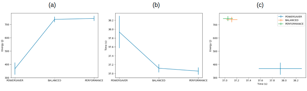 Figure 1. (a) Energy consumption in Joule of each power profile; (b) Processing time in seconds of each power profile; (c) Time vs Energy of each profile displayed in order to identify the Pareto frontier.
However to draw any conclusive interpretation we need to understand the statistical significance of the results. To do that we explored the data distribution using a box plot and a violin plot.
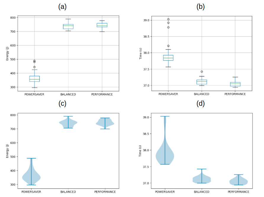
Figure 2. (a-b) Boxplots and (c-d) Violinplots to identify outliers and the distributions of the energy consumptions and processing times of the power profiles.
To run the necessary test for statistical significance we needed to confirm that the data is normal. As seen in the distribution plots this is hard to conclude just from the visualizations.
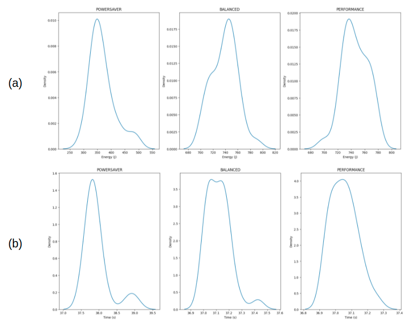
Figure 3. Kernel density plots to further highlight the nature of the data distributions for energy (a) and time (b) consumptions of each profile.
We therefore run a Shapiro-Wilk test to confirm normality. The p-values obtained from the tests are displayed in the following table.
| Powersaver Energy | Balanced Energy | Performance Energy | Powersaver Time | Balanced Time | Performance Time | |
|---|---|---|---|---|---|---|
| \(0.005\) | \(0.413\) | \(0.346\) | \(4\cdot 10^{-6}\) | \(0.009\) | \(0.239\) |
Table 2. p-values for the Shapiro-Wilk test performed on the obtained data.
As can be seen not all data is normally distributed at a significance level of 5%. We therefore tried to remove the outliers using z-scores, by removing points with a score higher than three standard deviations. However, only the time data for the Balanced profile became normal after outlier removal. We therefore performed a sanity check by rerunning the whole experiment for every profile. However, we got similar results and the data distributions that were not normal generally remained not normal, as can be seen in the following table.
| Powersaver Energy | Balanced Energy | Performance Energy | Powersaver Time | Balanced Time | Performance Time | |
|---|---|---|---|---|---|---|
| \(0.003\) | \(0.130\) | \(0.104\) | \(3\cdot 10^{-6}\) | \(0.094\) | \(6\cdot 10^{-5}\) |
Table 3. p-values for the Shapiro-Wilk test performed on the data obtained from running the experiments a second time.
Therefore we moved forward concluding that not all data distributions are normal.
Statistical Significance and Effect Size
Since we are comparing three different datasets for energy and time, one for each profile, we used the Bonferroni Correction to adjust the significance level for the statistical tests we conducted. Since we tested for a significance level of 0.05 and performed in each case, time and energy, 3 different tests, the corrected level was given by 0.05/3, which is 0.01667. We then checked the statistical significance of the differences between the three profiles by using a two-sided Welsch t-test or Manney-Wittney U-test depending on the normality of the data.
| Welsch t-test Performance vs Balanced | Manney-Wittney U-test Powersaver vs Balanced | Manney-Wittney U-test Powersaver vs Balanced |
|---|---|---|
| \(0.158\) | \(3\cdot 10^{-11}\) | \(3\cdot 10^{-11}\) |
Table 4. p-values for the statistical significance of the pair-wise differences between the energy data.
| Welsch t-test Performance vs Balanced | Manney-Wittney U-test Powersaver vs Balanced | Manney-Wittney U-test Powersaver vs Balanced |
|---|---|---|
| \(0.010\) | \(3\cdot 10^{-11}\) | \(3\cdot 10^{-11}\) |
Table 5. p-values for the statistical significance of the pair-wise differences between the time data.
Of these results, only the difference in energy consumption between the Balanced and Performance profile is not significant. We therefore moved to check first the difference in medians between the energy consumption of the Performance and Powersaver profile, which is 387 J, and between the Balanced and Powersaver profile, which is 386 J. In both cases, the difference is of three orders of magnitude. The difference in time, instead, is always below 1 second.
| Balanced - Powersaver (Median) Energy | Performance - Powersaver (Median) Energy | Balanced - Performance (Mean) Time | Powersaver - Balanced (Median) Time | Powersaver - Performance (Median) Time | |
|---|---|---|---|---|---|
| \(386.66\) | \(387.66\) | \(0.054\) | \(0.717\) | \(0.790\) |
Table 6. Pair-wise median or mean difference between the data, depending on the normality of the data.
We then computed the percentage change or the pairwise difference between the data, with the pairwise difference computed as the percentage of data pairs where the first element is greater than the second.
| Balanced - Powersaver Energy (Pairwise Difference) | Performance - Powersaver Energy (Pairwise Difference) | Balanced - Performance Time (Percentage Change) | Powersaver - Balanced Time (Pairwise Difference) | Powersaver - Performance Time (Pairwise Difference) | |
|---|---|---|---|---|---|
| 100% | 100% | 14% | 100% | 100% |
Table 7. Pair-wise median or mean difference between the data, depending on the normality of the data.
Finally, we computed the Choen’s or Cliff’s delta, again depending on the normality of the data. Each Cliff’s delta result indicated that the difference of the distributions is large, each with a score of 1. In the case of the times of the Balanced and Performance profile, Choen’s delta also indicated that the distributions are separated, with a score of 0.985, signifying a separation of almost an entire standard deviation.
Practical Significance and Further Results
What are results show is that the difference in energy saving between the Balanced and Performance profiles is not statistically significant, while the energy savings obtained by the Powersaver profile compared to the other two profiles are significant. Looking at the median difference we can see that the energy savings obtained by the Powersaver profile are almost half of the entire energy consumption of the other two profiles.
Looking at the processing time data we also notice that the effect size metrics point to a great degree of separation. However, by investigating the mean and median differences we can see that the magnitude of these separations is within a single second. Therefore while statistically significant the results on time do not indicate a clear preferred profile to use in a real-world scenario.
We performed the same tests also for the second run of experiments, with results confirming the ones here presented. Furthermore we executed the same experiment also on the CPU to see if the results would transfer also to that setting. What we found, again, is that while the Powersaver profile saves significant amounts of energy, no profile dominates the others by a significant magnitude in terms of processing time.
All our notebooks containing the analysis for each set of experiments can be found at our github repository.
Discussion
The presented work comes with a couple of limitations. The Perfzero TensorFlow benchmark tool requires an internet connection to be able to run. An Internet connection can cause serious distortions in the measurement, for instance, due to background processes that need to sync. Another limitation related to the benchmark tool is that we chose a synthetic benchmark tool to keep the experiments short. Real-world machine learning training jobs in common scenarios can take several hours to complete. In an ideal experiment, such a real-world training job would be the best choice. Another limitation is that ultimately, the effects of the unwanted side factors cannot be removed. These factors, especially in our setup, can only be minimized. Lastly, the gathered data does not follow a normal distribution for all power profile results. However, it is known that when working with AI applications, the outcome is rarely deterministic and a normal distribution is therefore not always feasible.
In the context of our research, the Powersaver profile is the most energy-efficient. However, in a real scenario, a user might not do the same preparation as we did. They might have their screen turned on, or unnecessary background processes running. As stated earlier, looking at the whole pipeline for ML applications is important [7]. Since the Powersaver profile has an overall longer runtime, it could be possible that with additional energy-consuming processes running for an overall longer time, the Powersaver profile might be more energy-consuming than the other energy profiles. Extra research needs to be conducted to prove or disprove this hypothesis.
Furthermore, we found that the difference in time between the profiles is not in a relevant order of magnitude. However, the effect size clearly indicates that the results obtained by each profile are statistically separated. Since we performed our test under a simple benchmark we cannot, therefore, be sure how the processing times scale under a more complex benchmark. It is possible that while in our case the differences are between a second, these differences can scale to hours or more under a more complex task.
Finally, the use of a simple benchmark might have hidden the real differences between the Balanced and Performance energy consumptions. While we found that these were not statistically significant, under a more complex task the difference could become significant as the CPU or GPU will need more resources for a longer time. Lastly, Performance mode can be hardware or battery level dependent, which makes it hard to accurately measure performance.
Conclusion
In this work, we have motivated the need for energy-efficient solutions, especially in energy-intensive domains like ML. One easy way to adjust the power usage on laptops is by applying different power profiles. Three different power profiles for Ubuntu have been benchmarked on an ML training benchmark job. The experiments measured both energy consumption and the runtime of the training job. The results of the experiments show that the Powersaver profile consumes significantly less energy than the Balanced and Performance profiles. While the runtime shows the same significant difference, the practical significance is less applicable. The small increase in runtime compared to the large decrease in energy consumption makes the Powersaver profile a viable energy-aware choice for ML engineers. The experiments were repeated with Tensorflow without GPU support. A similar energy pattern emerged, with again little practical significance in the difference in runtime across all power profiles. Further research can extend this work by repeating the experiments in a more controlled setting. Furthermore, instead of short synthetic benchmarks, real benchmarks can be used to simulate real-world ML model training scenarios. At last, different systems can be evaluated including operating systems, different models and datasets, and different types of hardware including hardware that is more commonly used by ML engineers.
References
[1] Hayri Acar, G ̈ulfem I Alptekin, Jean-Patrick Gelas, and Parisa Ghodous. The Impact of Source Code in Software on Power Consumption. International Journal of Electronic Business Management, 14:42–52, 2016.
[2] Coral Calero and Mario Piattini. Introduction to Green in Software Engineering, pages 3–27. Springer International Publishing, Cham, 2015.
[3] Eva Garc ́ıa-Mart ́ın, Crefeda Faviola Rodrigues, Graham Riley, and H ̊akan Grahn. Estimation of energy consumption in machine learning. Journal of Parallel and Distributed Computing, 134:75–88, 2019.
[4] Erik Jagroep, Jan Martijn E. M. van der Werf, Slinger Jansen, Miguel Ferreira, and Joost Visser. Profiling energy profilers. In Proceedings of the 30th Annual ACM Symposium on Applied Computing, SAC ’15, page 2198–2203, New York, NY, USA, 2015. Association for Computing Machinery.
[5] Mohit Kumar, Xingzhou Zhang, Liangkai Liu, Yifan Wang, and Weisong Shi. Energy-efficient machine learning on the edges. In 2020 IEEE International Parallel and Distributed Processing Symposium Workshops (IPDPSW), pages 912–921, 2020.3
[6] Stefan Naumann, Markus Dick, Eva Kern, and Timo Johann. The greensoft model: A reference model for green and sustainable software and its engineering. Sustainable Computing: Informatics and Systems, 1(4):294–304, 2011.
[7] Carole-Jean Wu, Ramya Raghavendra, Udit Gupta, Bilge Acun, Newsha Ardalani, Kiwan Maeng, Gloria Chang, Fiona Aga, Jinshi Huang, Charles Bai, Michael Gschwind, Anurag Gupta, Myle Ott, Anastasia Melnikov, Salvatore Candido, David Brooks, Geeta Chauhan, Benjamin Lee, Hsien-Hsin Lee, Bugra Akyildiz, Maximilian Balandat, Joe Spisak, Ravi Jain, Mike Rabbat, and Kim Hazelwood. Sustainable ai: Environmental implications, challenges and opportunities. In D. Marculescu, Y. Chi, and C. Wu, editors, Proceedings of Machine Learning and Systems, volume 4, pages 795–813, 2022.
[8] Wenninger, Simon; Kaymakci, Can; Wiethe, Christian; Römmelt, Jörg; Baur, Lukas; Häckel, Björn; and Sauer, Alexander, “How Sustainable is Machine Learning in Energy Applications? – The Sustainable Machine Learning Balance Sheet” (2022). Wirtschaftsinformatik 2022 Proceedings.
[9] SA Budennyy, VD Lazarev, NN Zakharenko, AN Korovin, OA Plosskaya, DV Dimitrov, VS Akhripkin, IV Pavlov, IV Oseledets, IS Barsola, et al. Eco2ai: carbon emissions tracking of machine learning models as the first step towards sustainable ai. In Doklady Mathematics, pages 1–11. Springer, 2023.